Lesson 21: Invoice, Part 2: Using VLOOKUP
/en/excelformulas/invoice-part-1-free-shipping/content/

"Say…you know, you did such a nice job figuring out that free shipping formula, I thought I'd throw this your way.
We're starting to process a lot more invoices these days. It gets tedious to look up the product name and price from the Products worksheet after adding the product ID. Do you know if there's a way to have our spreadsheet pull in this info automatically?"
This lesson is part 2 of 5 in a series. You can go to Invoice, Part 1: Free Shipping if you'd like to start from the beginning.
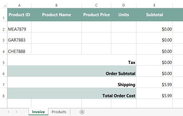
Our spreadsheet
Once you've downloaded our spreadsheet, open the file in Excel or another spreadsheet application. It looks similar to the invoice from the last lesson, but now we have two different worksheets: one for the Invoice, and one for the Products.
What are we trying to do with this spreadsheet?
Our coworker asked if we could use the Product ID number to find the the product name and price from the Products worksheet. Luckily, the VLOOKUP function can do this automatically. If you've never used VLOOKUP before, don't worry—we'll show you how to use it below.
VLOOKUP is a bit more advanced than some functions, so you'll need to be familiar with functions and cell references before you begin. You can review our lessons on Functions and Relative and Absolute Cell References to learn more.
How it works
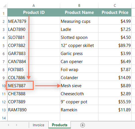
Before we start using VLOOKUP, it will be helpful to know what it does. In our example, it will search for the Product ID number on the Products worksheet. It first searches vertically down the first column (VLOOKUP is short for "vertical lookup"). When it finds the desired product ID, it moves to the right to find the product name and product price.
Before we write our function, we'll need to take a moment to think carefully about each argument and collect some information from our spreadsheet. The arguments will tell VLOOKUP what to search for and where to look. We'll need to use four arguments:
- The first argument tells VLOOKUP what to search for. In our example, we're searching for the product ID number, which is in cell A2, so our first argument is A2.
- The second argument is a cell range that tells VLOOKUP where to look for the value from our first argument. In our example, we want it to search for this value in cell range A2:C13 on the Products worksheet, so our second argument is Products!$A$2:$C$13. Note that we're using absolute references so this range won't change when we copy the formula to other cells.
- The third argument is the column index number, which is simpler than it sounds: The first column in the cell range from the previous argument is 1, the second column is 2, and so on. In our example, we're looking for the Product Name. The names are stored in the second column of the cell range from the previous argument, so our our third argument is 2.
- The fourth argument tells VLOOKUP if it should look for approximate or exact matches. If it is TRUE, it will look for approximate matches. If it is FALSE, it will look for exact matches. In this example, we're only looking for exact matches, so our fourth argument is FALSE.
It's important to know that VLOOKUP will always search the leftmost column in the cell range. Since our cell range is A2:C13, it will search column A.
Writing the function
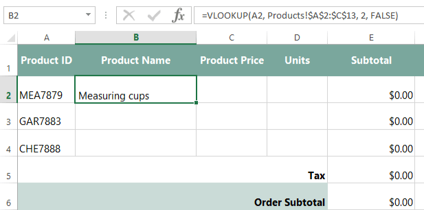
Now that we have our arguments, we'll write our function in cell B2. We'll start by typing an equals sign (=), followed by the function name and an open parenthesis:
=VLOOKUP(
Next, we'll add each of the four arguments, separate them with commas, then close the parentheses:
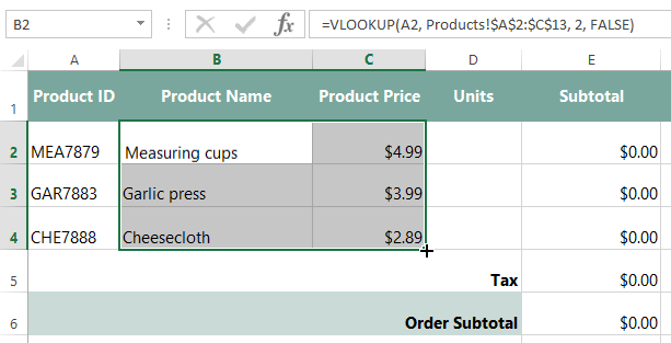
=VLOOKUP(A2, Products!$A$2:$C$13, 2, FALSE)
If you entered the function correctly, the product name should appear: Measuring cups. If you want to test your function, change the Product ID number in cell A2 from MEA7879 to CHE7888. The product name should change from Measuring cups to Cheesecloth.
Note: Be sure to type the product ID exactly as it appears above, with no spaces. Otherwise, the VLOOKUP function will not work correctly.
Adding the product price
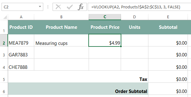
Next, we also want the Product ID to pull in the product price, so we'll use the VLOOKUP function again. Since we're using the same data, this function will be very similar to the one we just added. In fact, all we have to do is change the third argument to 3. This will tell VLOOKUP to pull in the data from the third column, where the product price is stored:
=VLOOKUP(A2, Products!$A$2:$C$13, 3, FALSE)
OK, let's enter our new formula in cell C2:
We've got our formulas working, so we can just select cells B2 and C2 and then drag the fill handle down to copy the formulas to the other rows in the invoice. Now, each row is using VLOOKUP to find the Product Name and Product Price.
OK—our functions look good. Let's send this back!

"Excellente! This is going to save the invoice team a boatload of time each day.
You're really a whiz with this kind of stuff! Thanks a bunch!"
Bonus Section
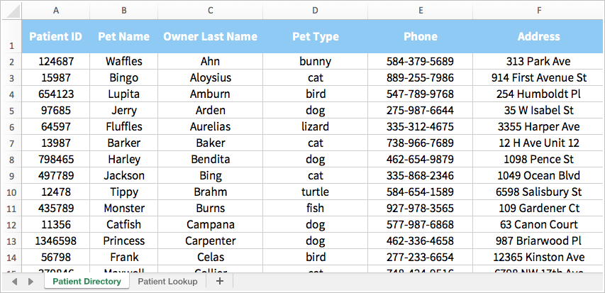
Let's say a veterinarian's office is creating a spreadsheet to look up patient information.
Here's the patient directory. This is where information will be pulled from:
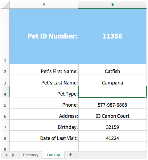
Here's the patient lookup sheet. This is where the function will be inserted.
If you'd like to continue on to the next part in this series, go to Invoice, Part 3: Fix Broken VLOOKUP.
/en/excelformulas/invoice-part-3-fix-broken-vlookup/content/