Excel: Freezing Panes and View Options

Lesson 18: Freezing Panes and View Options

/en/excel/basic-tips-for-working-with-data/content/

Introduction

Whenever you're working with a lot of data, it can be difficult to compare information in your workbook. Fortunately, Excel includes several tools that make it easier to view content from different parts of your workbook at the same time, including the ability to freeze panes and split your worksheet.

Optional: Download our practice workbook.

Watch the video below to learn more about freezing panes in Excel.

To freeze rows:

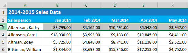
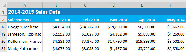
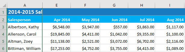
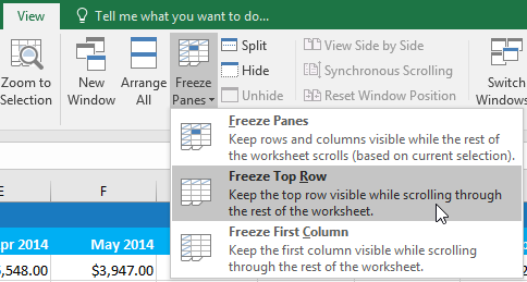
You may want to see certain rows or columns all the time in your worksheet, especially header cells. By freezing rows or columns in place, you'll be able to scroll through your content while continuing to view the frozen cells.

  1. Select the row below the row(s) you want to freeze. In our example, we want to freeze rows 1 and 2, so we'll select row 3.
    Selecting cells
  2. On the View tab, select the Freeze Panes command, then choose Freeze Panes from the drop-down menu.
    The Freeze Rows dropdown menu
  3. The rows will be frozen in place, as indicated by the gray line. You can scroll down the worksheet while continuing to view the frozen rows at the top. In our example, we've scrolled down to row 18.
    The top two rows are now frozen data

To freeze columns:

  1. Select the column to the right of the column(s) you want to freeze. In our example, we want to freeze column A, so we'll select column B.
    selecting column B
  2. On the View tab, select the Freeze Panes command, then choose Freeze Panes from the drop-down menu.
    /content/561fbc87287fc10e146dbf44_10_15_2015/freeze-rows-dropdown-menu.png
  3. The column will be frozen in place, as indicated by the gray line. You can scroll across the worksheet while continuing to view the frozen column on the left. In our example, we've scrolled across to column E.
    The first column is now frozen

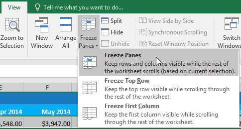
If you only need to freeze the top row (row 1) or first column (column A) in the worksheet, you can simply select Freeze Top Row or Freeze First Column from the drop-down menu.

The Freeze Top Row command

To unfreeze panes:

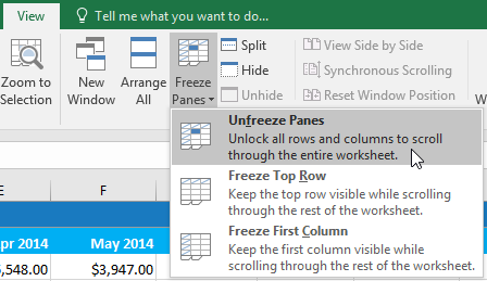
If you want to select a different view option, you may first need to reset the spreadsheet by unfreezing panes. To unfreeze rows or columns, click the Freeze Panes command, then select Unfreeze Panes from the drop-down menu.

The Unfreeze Panes command

Other view options

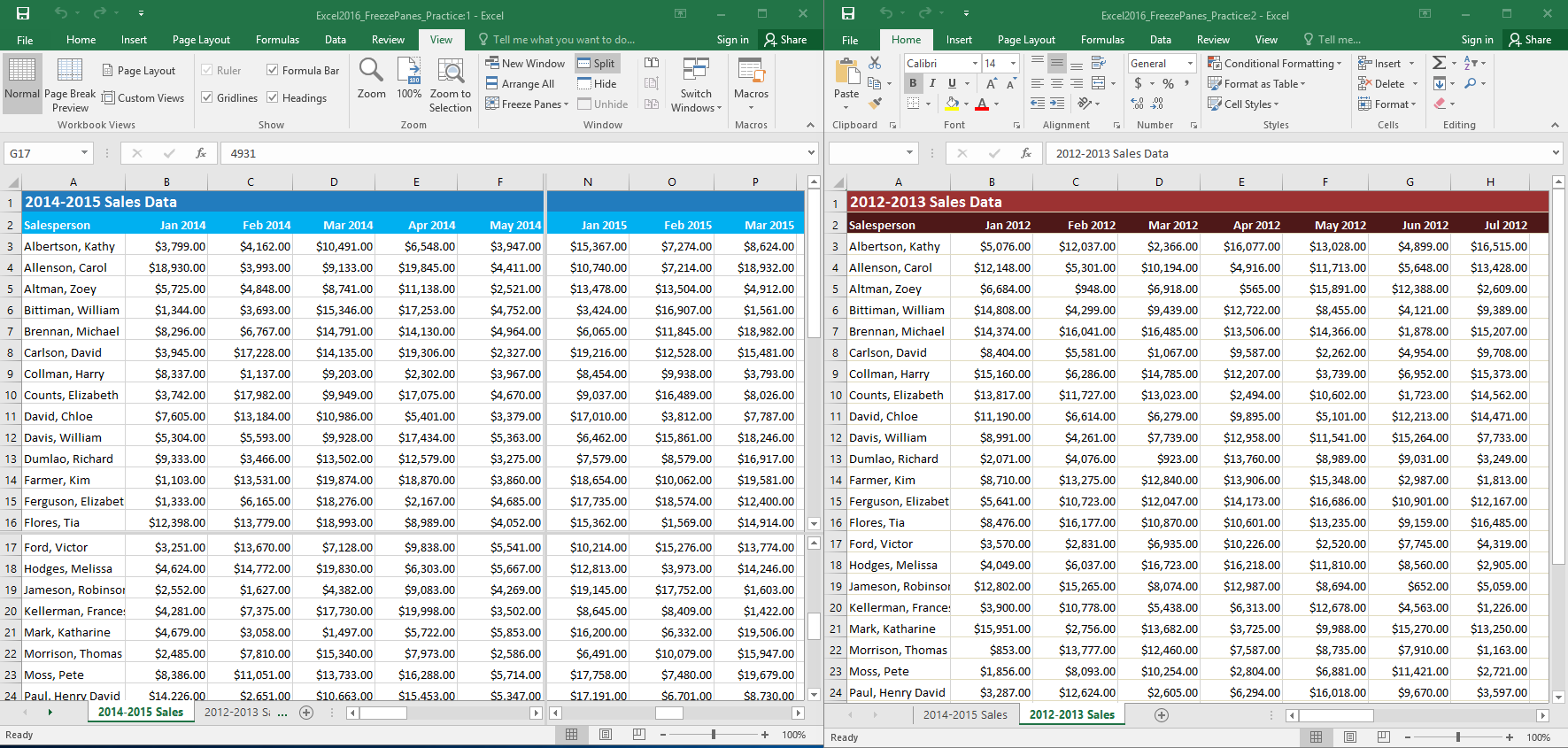
If your workbook contains a lot of content, it can sometimes be difficult to compare different sections. Excel includes additional options to make your workbooks easier to view and compare. For example, you can choose to open a new window for your workbook or split a worksheet into separate panes.

To open a new window for the current workbook:

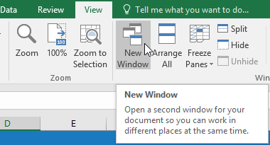
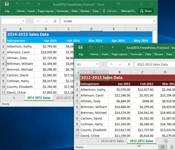
Excel allows you to open multiple windows for a single workbook at the same time. In our example, we'll use this feature to compare two different worksheets from the same workbook.

  1. Click the View tab on the Ribbon, then select the New Window command.
    The New Window button on the View tab
  2. A new window for the workbook will appear.
    Two windows for the same workbook
  3. You can now compare different worksheets from the same workbook across windows. In our example, we'll select the 2013 Sales Detailed View worksheet to compare 2012 and 2013 sales.
    You can compare different parts of the same workbook

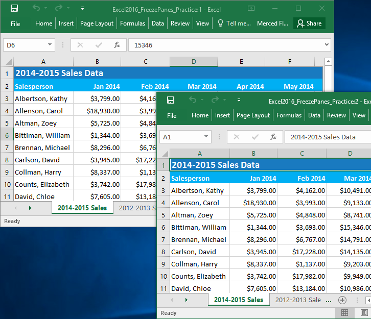
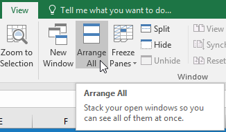
If you have several windows open at the same time, you can use the Arrange All command to rearrange them quickly.

The Arrange All button on the View tab

To split a worksheet:

Sometimes you may want to compare different sections of the same workbook without creating a new window. The Split command allows you to divide the worksheet into multiple panes that scroll separately.

  1. Select the cell where you want to split the worksheet. In our example, we'll select cell D6.

    Selecting cells

  2. Click the View tab on the Ribbon, then select the Split command.
    The Split command on the View tab
  3. The workbook will be split into different panes. You can scroll through each pane separately using the scroll bars, allowing you to compare different sections of the workbook.
    Scrolling through split panes
  4. After creating a split, you can click and drag the vertical and horizontal dividers to change the size of each section.

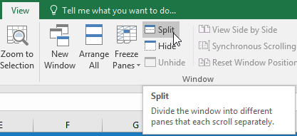
To remove the split, click the Split command again.

Challenge!

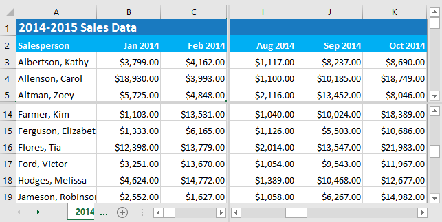
Within our example file, there is A LOT of sales data. For this challenge, we want to be able to compare data for different years side by side. To do this:

  1. Open our practice workbook.
  2. Open a new window for your workbook.
  3. Freeze First Column and use the horizontal scroll bar to look at sales from 2015.
  4. Unfreeze the first column.
  5. Select cell G17 and click Split to split the worksheet into multiple panes. Hint: This should split the worksheet between rows 16 and 17 and columns F and G.
  6. Use the horizontal scroll bar in the bottom-right of the window to move the worksheet so Column N, which contains data for January 2015, is next to Column F.
  7. Open a new window for your workbook and select the 2012-2013 Sales tab.
  8. Move your windows so they are side by side. Now you're able to compare data for similar months from several different years. Your screen should look something like this:
    Freezing Panes Challenge

/en/excel/sorting-data/content/